Chapter 4 System of Linear Equations
Section 4.2 LS in two Variables4.2.1 Introduction
At first we will restrict ourselves to systems of linear equations in two variables.
Generally, a system of linear equations (LS) consisting of two equations in the variables and has the following structure:
Here, , and are the so-called coefficients of the system of linear equations, which are, as and on the right-hand sides of the equations, often real numbers given by the problem description. If the right-hand sides and both are equal to (), the system of linear equations is called homogeneous, and inhomogeneous otherwise.
Because of their linearity, each of the two equations of the system in info box 4.2.1 can be interpreted as the equation of a line in the --plane. If, for example, the first equation is solved for ,
one immediately sees from this explicit form that it describes a line with the slope and the -intercept .
Note that solving the equation for is only allowed if . For , the first equation reads ; for this is equivalent to , i.e. is a constant. This equation also describes a line, namely a line parallel to the -axis with -intercept .
And what about the case in which both and ? Then, we also have , since otherwise the first equation would result in a contradiction. But for , the first equation is (for all values of and ) always identically satisfied (), and hence useless.
The case of the second equation in info box 4.2.1 is similar:
Altogether, one obtains two lines representing the two linear equations. The question for the solvability and for the solution of the system of linear equations, namely the question for the simultaneous validity of the two equations reads as the question for the existence and the position of the intersection point of the two lines. To this, let us investigate a specific example.
This intuitive approach is very well suited to discussing all cases which can generally occur: two lines in the --plane can intersect each other - and then the intersection point is necessarily unique -, or the two lines are parallel and thus do not have any intersection point, or the two lines coincide - so to speak - they intersect in an infinite number of points. There are no other cases.
Accordingly, the corresponding system of linear equations has one of the following solution sets:
An inhomogeneous system of linear equations has either one unique solution, no solution, or an infinite number of solutions.
An homogeneous system of linear equations has always at last one solution, namely the so-called trivial solution , . Moreover, such a homogeneous system can also have an infinite number of solutions.
This will be illustrated by two further examples starting directly with the systems of linear equations: For the example on the right, other parametrisations of the solution set are possible and allowed. It basically just depends on how to describe the points of the (congruent) lines appropriately. The above description of the solution set simply used the equation of the line itself and the control variable was denoted by instead of .
And what about the above mentioned restrictions due to the base set? Let us look at the following example.
Info 4.2.1
Generally, a system of linear equations (LS) consisting of two equations in the variables and has the following structure:
Here, , and are the so-called coefficients of the system of linear equations, which are, as and on the right-hand sides of the equations, often real numbers given by the problem description. If the right-hand sides and both are equal to (), the system of linear equations is called homogeneous, and inhomogeneous otherwise.
Because of their linearity, each of the two equations of the system in info box 4.2.1 can be interpreted as the equation of a line in the --plane. If, for example, the first equation is solved for ,
one immediately sees from this explicit form that it describes a line with the slope and the -intercept .
Note that solving the equation for is only allowed if . For , the first equation reads ; for this is equivalent to , i.e. is a constant. This equation also describes a line, namely a line parallel to the -axis with -intercept .
And what about the case in which both and ? Then, we also have , since otherwise the first equation would result in a contradiction. But for , the first equation is (for all values of and ) always identically satisfied (), and hence useless.
The case of the second equation in info box 4.2.1 is similar:
Altogether, one obtains two lines representing the two linear equations. The question for the solvability and for the solution of the system of linear equations, namely the question for the simultaneous validity of the two equations reads as the question for the existence and the position of the intersection point of the two lines. To this, let us investigate a specific example.
Example 4.2.2
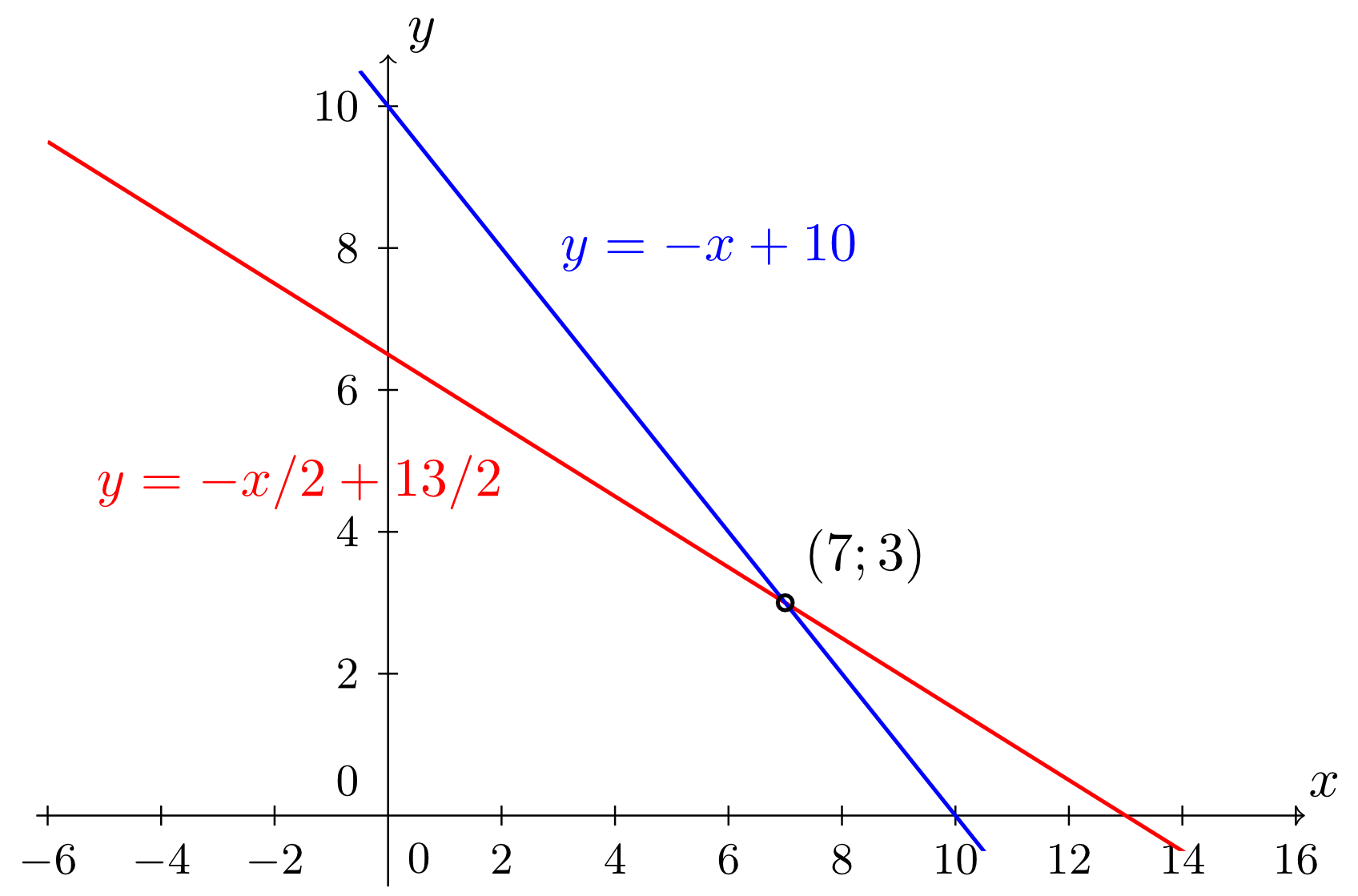
The system of linear equations in the first example 4.1.1 reads:
(Here, the general coefficients and right-hand sides of the system 4.2.1 have the specific values , and .)
The equations describe two lines with the slopes and , respectively, and the -intercepts and , respectively.
The figure shows that the two lines do indeed intersect, and one reads off the coordinates of the intersection point as . Accordingly, the system of linear equations considered here has a unique solution. The solution set consists of exactly one pair of numbers, namely .
This intuitive approach is very well suited to discussing all cases which can generally occur: two lines in the --plane can intersect each other - and then the intersection point is necessarily unique -, or the two lines are parallel and thus do not have any intersection point, or the two lines coincide - so to speak - they intersect in an infinite number of points. There are no other cases.
Accordingly, the corresponding system of linear equations has one of the following solution sets:
Info 4.2.3
An inhomogeneous system of linear equations has either one unique solution, no solution, or an infinite number of solutions.
An homogeneous system of linear equations has always at last one solution, namely the so-called trivial solution , . Moreover, such a homogeneous system can also have an infinite number of solutions.
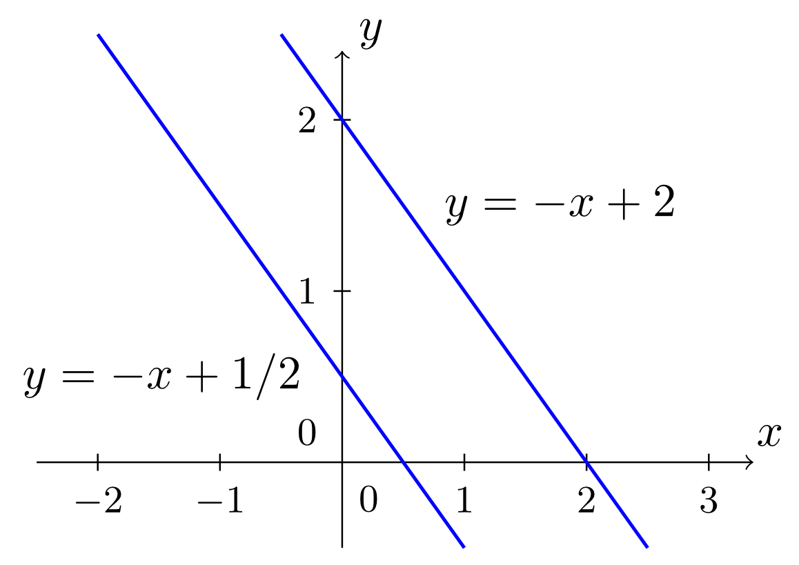
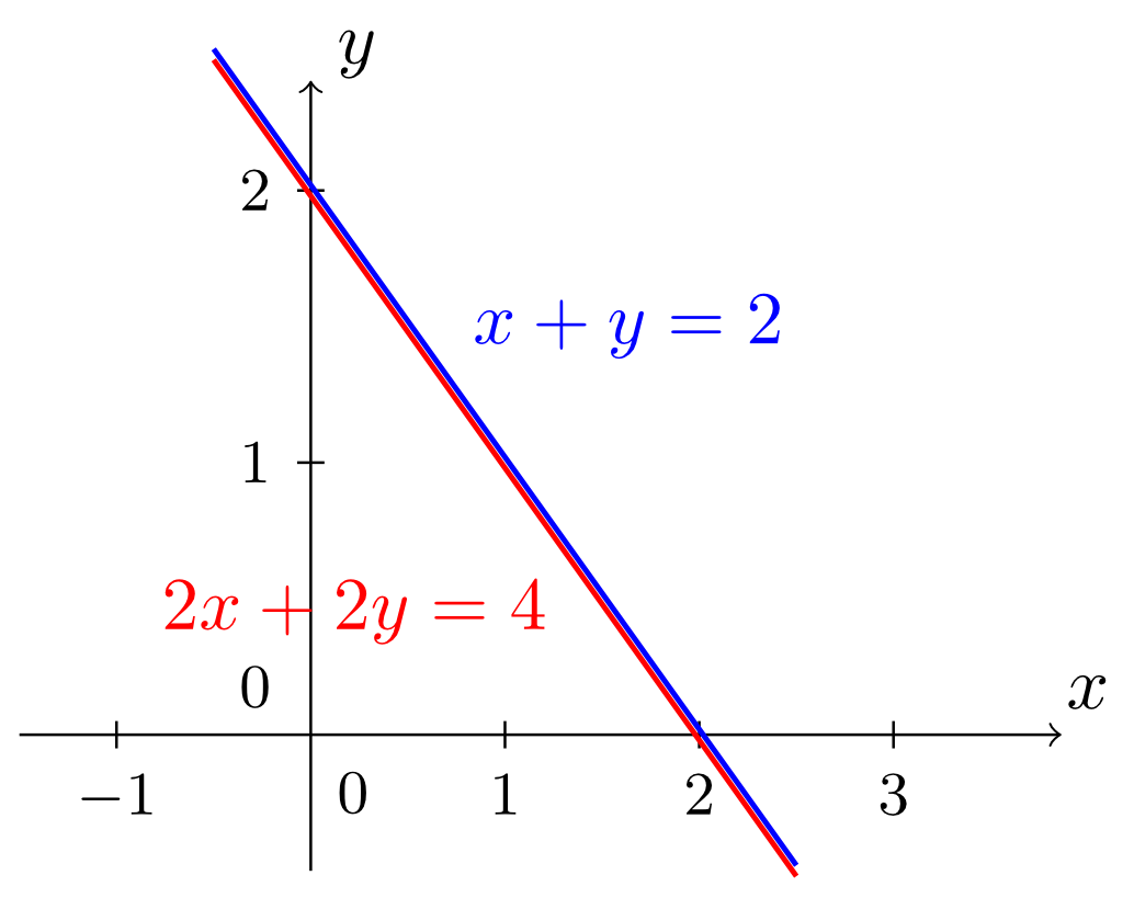
This will be illustrated by two further examples starting directly with the systems of linear equations:
Example 4.2.4
In both cases the base set is the set of the real numbers .
And what about the above mentioned restrictions due to the base set? Let us look at the following example.
Example 4.2.5
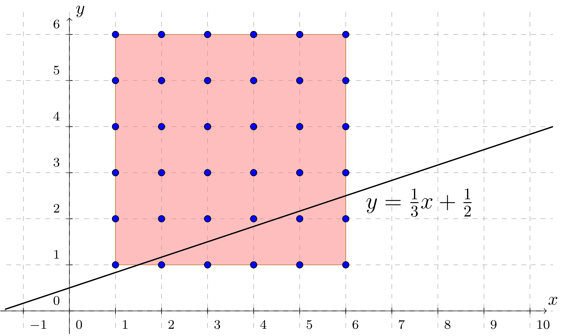
At a local fair, an exceptionally clever stallholder promises almost dreamlike prizes for an absurdly low initial wager if one, yes, only one of the passers-by is able to unravel the following little mystery:
I rolled a die twice. If I subtract twice the first number I rolled from six times the second number, I get the number . If I add to four times the first number, I get the twelve times the second number. Which two numbers did I roll?
Let the first number he rolled be denoted by and the second by . Then the statements of the stallholder can be translated very quickly into a set of equations:
One realises that the corresponding system of linear equations - interpreted geometrically - results in two congruent lines. At first glance, it thus seems to have an infinite number of solutions.
But now the base set has to be taken into account: since both and represent numbers on a die, the two variables can only take values from the set . If one looks at the line in the --plane, one sees that no possible pair of numbers thrown on a die fall onto this line. Hence, the solution set in this case is indeed the empty set .