Chapter 8 Integral Calculus
Section 8.2 Definite Integral8.2.2 Integral
The integral of a function with can be interpreted as the "area under the graph" of the function. In the so-called Riemann integral, the graph of the function is approximated by a step function, and the values of this step function are summed up, weighted by the corresponding interval length, i.e. the "width of a step". This approach is illustrated in the figure below.
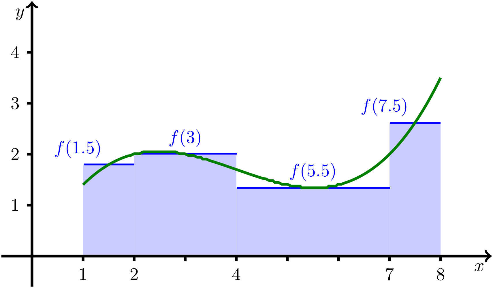
Definition of the Riemann integral. The function is approximated by a step function that is divided here into four subintervals.
Formally, a sum of the form
is calculated. In the example considered here, the interval is divided into four parts, where , , , and . If the areas of these four parts are summed according to the formula above, this results in
To get precise values for the area, it is obviously not sufficient to subdivide the interval into just a few subintervals. In general, it will be necessary to decrease the maximal length of the subintervals gradually, which in turn requires more summands to be calculated and added. Hence, the limit is considered as the maximal length of the subintervals tends to zero.
In principle, the approach discussed above can also be applied to functions with negative function values. We will explain in Section 8.3 how the area is calculated then. However, note that in the definition of the integral a few aspects have to be observed that go beyond the scope of this course. Therefore, we refer to advanced textbooks for details concerning the assumptions in the definitions below.
Integral 8.2.1
Let a function on a real interval be given. If the number of subintervals is increased such that approaches , then
is called the definite integral of with the lower limit of integration and the upper limit of integration (if the limit exists and does not depend on the respective partition). The function is then referred to as integrable. In this context the function is also called the integrand.
In principle, this approach can also result in an indefinite value, i.e. the integral does not exist. However, advanced considerations show that the integral exists for every continuous function. As an example, we calculate the integral of , where we focus on the calculation of the limit.
The large class of integrable functions includes all polynomials, rational functions, trigonometric functions, exponential functions, logarithmic functions and their compositions.
To simplify the calculations, rules for integrating functions are required that are as easy as possible. An important result is provided by the so-called fundamental theorem of calculus. It describes the relation between the antiderivative of a continuous function and its integral.
As a simple example, we will calculate the definite integral of the function with between and . Using the rules for the determination of antiderivatives and the fundamental theorem of calculus this problem can be solved easily.
The equation in the fundamental theorem also applies to every intermediate value such that all function values can be calculated from
if the derivative and a function value, for example the value , are known. One also says that the antiderivative is reconstructed from the derivative .
Application examples for the reconstruction of a function from its derivative are discussed at the end of Section 8.3.
is called the definite integral of with the lower limit of integration and the upper limit of integration (if the limit exists and does not depend on the respective partition). The function is then referred to as integrable. In this context the function is also called the integrand.
In principle, this approach can also result in an indefinite value, i.e. the integral does not exist. However, advanced considerations show that the integral exists for every continuous function. As an example, we calculate the integral of , where we focus on the calculation of the limit.
Example 8.2.2
Calculate the integral of .
For this purpose, the interval is subdivided into subintervals of equal length with and . Thus, the length of a subinterval is .
Investigating the length of the interval for tending to infinity shows that is getting smaller and approaches zero. Thus, the assumption for the calculation of a definite integral is satisfied.
Furthermore, for the values of , we obtain from the length of an interval . If we set for the intermediate points, we obtain .
Substituting these terms into the formula (1) gives the equation
where we used the formula of Carl Friedrich Gauss. And with , we find for the integral
The large class of integrable functions includes all polynomials, rational functions, trigonometric functions, exponential functions, logarithmic functions and their compositions.
To simplify the calculations, rules for integrating functions are required that are as easy as possible. An important result is provided by the so-called fundamental theorem of calculus. It describes the relation between the antiderivative of a continuous function and its integral.
As a simple example, we will calculate the definite integral of the function with between and . Using the rules for the determination of antiderivatives and the fundamental theorem of calculus this problem can be solved easily.
Example 8.2.4
The function with has the antiderivative with
for a real number . From the fundamental theorem, we have
The calculation shows that the constant is cancelled after substituting the lower and upper limits of integration such that, in practice, it can already be "suppressed" in taking the antiderivative for the definite integral, so for the calculation of the definite integral one can choose .
The equation in the fundamental theorem also applies to every intermediate value such that all function values can be calculated from
if the derivative and a function value, for example the value , are known. One also says that the antiderivative is reconstructed from the derivative .
Application examples for the reconstruction of a function from its derivative are discussed at the end of Section 8.3.
:
