7.5.2 Chapter 7 Differential Calculus
Section 7.5 Applications7.5.1 Curve Analysis
Curve analysis is an established part of the German mathematics syllabus that consists of curve sketching for a function together with the gathering of certain standardized qualitative and quantitative information about the function graph.
Let a differentiable function with the mapping rule for be given. In this course, a complete curve analysis of includes the following information:
- maximum domain
- - and -intercepts of the graph
- symmetry of the graph
- limiting behaviour/asymptotes
- first derivatives
- extremal values
- monotony behaviour
- inflexion points
- bending behaviour (curvature)
- sketch of the graph
Many of these points were already discussed in Module 6. Therefore, in this section we shall only briefly repeat what is meant by the different steps of curve analysis. Subsequently, we will discuss one example of a curve analysis in detail.
The first part of the curve analysis involves the algebraic and geometric aspects of :
- Maximum Domain
- All real numbers for which exists are determined. The set of these numbers is called the maximum domain.
- - and -Intercepts
-
- -axis: All zeros of are determined.
- -axis: The function value (if ) is calculated.
- -axis: All zeros of are determined.
- Symmetry of the Graph
- The graph of the function is symmetrical with respect to the -axis if for all . Then the function is called even. If for all , the graph is centrally symmetric with respect to the origin of the coordinate system. In this case, the function is called odd.
- Asymptotic Behaviour at the Domain Boundary
- The limits of the function at the boundaries of its domain are investigated.
In the second part, the function is investigated analytically by means of conclusions from the first derivatives. Of course, the first and the second derivative have to be calculated first, provided they exist.
- Derivatives
-
Calculation of the first and the second derivative (if they exist). - Extremal Values and Monotony
-
The necessary condition for to be an extremum (if is not a boundary point of ), is .
Thus, we calculate the points at which the derivative takes the value zero. If at these points also the second derivative exists, then we have:- : is a minimum point of .
- : is a maximum point of .
- : is a minimum point of .
- Inflexion Points and Curvature Properties
- The necessary condition for to be an inflexion point (if the second derivative exists), is
If and , then is an inflexion point, i.e. the bending behaviour of changes at this point.
The function is convex (left curved) on that intervals of the domain in which we have . It is concave (right curved) on that intervals on which we have . - Sketch of the Graph
- A sketch of the graph is drawn based on the information gained during the previous steps.
Detailed Example
We investigate a function defined by the mapping ruleMaximum Domain
The maximum domain of this function is since the denominator , i.e. it is always non-zero, and hence no points have to be excluded.
- and -Intercepts
The zeros of the function are the zeros of the numerator. Hence, the graph of intersects the -axis only at the origin since the numerator is only zero for . This is also the only intersection point with the -axis since there we have .
Symmetry
To investigate the symmetry we replace the argument by . We have
for all . Hence, the graph of the function is centrally symmetric with respect to the origin.
Limiting Behaviour
The function is defined on the entire set of real numbers , so only the limiting behaviour for and has to be investigated. Since is a fraction of two polynomials and the denominator has a greater power than the numerator, the -axis is a horizontal asymptote in both directions:
Derivatives
The first two derivatives of the function are calculated from the quotient rule. For the first derivative, we have:
Taking the derivative again and simplifying the terms results in:
Extremal Values
The necessary condition for an extremum at is , in this case . Thus, we obtain and . In addition, we have to investigate the behaviour of the second derivative at these points:
Hence, is a maximum point and is a minimum point of . Inserting these values for into results in the maximum point and the minimum point of .
Monotony Behaviour
Since is defined on the entire set of real numbers , the monotony behaviour can be derived from the position of the extremal points and their types: is monotonically decreasing on , monotonically increasing on , and monotonically decreasing on . Monotony intervals are always given as open intervals.
Inflexion Points
From the necessary condition for to be an inflexion point, we have the equation . Thus, , , and are the only solutions. The polynomial in the denominator of is always greater than zero. Since the polynomial in the numerator has only single roots, the second derivative changes its sign at all these points. Hence, these points are inflexion points of . The coordinates of the inflexion points , , are determined by inserting the corresponding values for into .
Bending Behaviour
The twice-differentiable function is convex if the second derivative is greater or equal to zero. It is concave if the second derivative is less or equal to zero. Since the polynomial in the denominator of is always positive, it is sufficient to examine the sign of the polynomial in the numerator. For , it is negative ( is concave there). For it is positive ( is convex there). Since is centrally symmetric, it follows that is convex on the intervals and and concave on the intervals and .
Sketch of the Graph
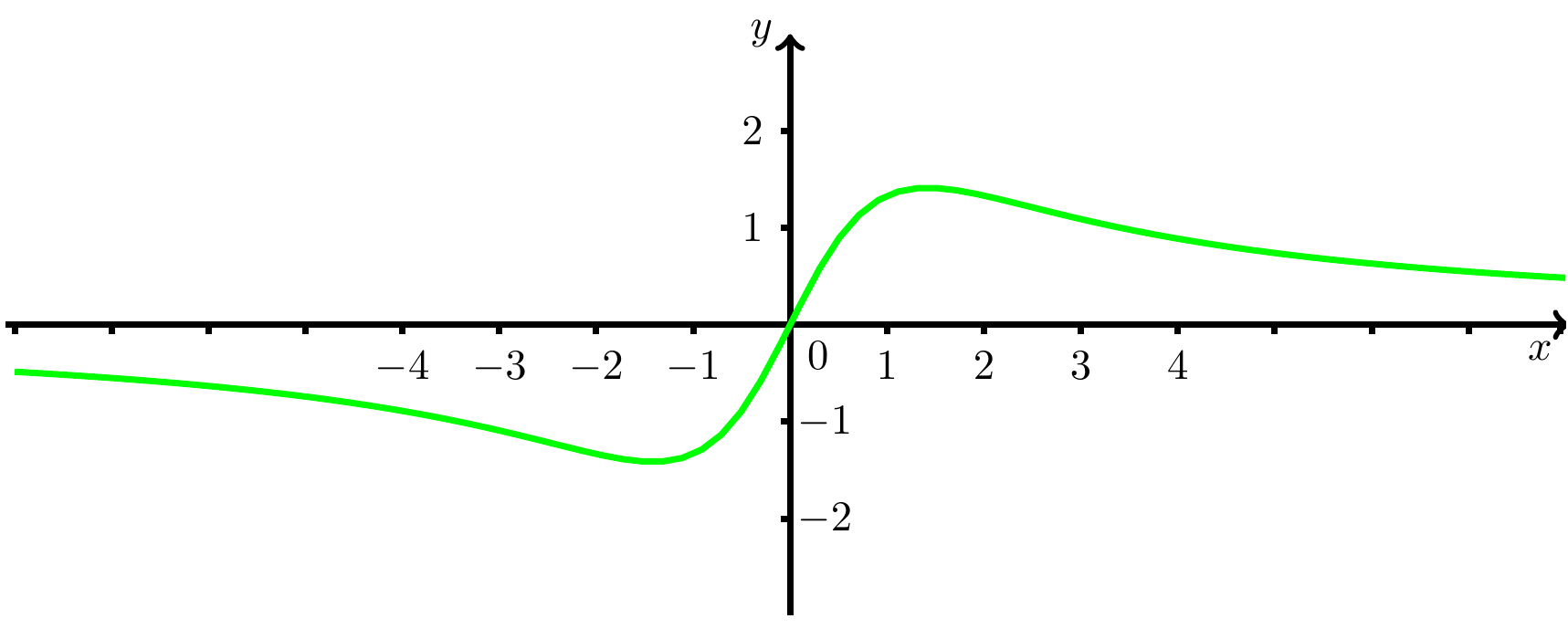
Abbildung 1: The graph of the function , sketched on the interval .
