Chapter 6 Elementary Functions
Section 6.2 Linear Functions and Polynomials6.2.7 Polynomials and Their Roots
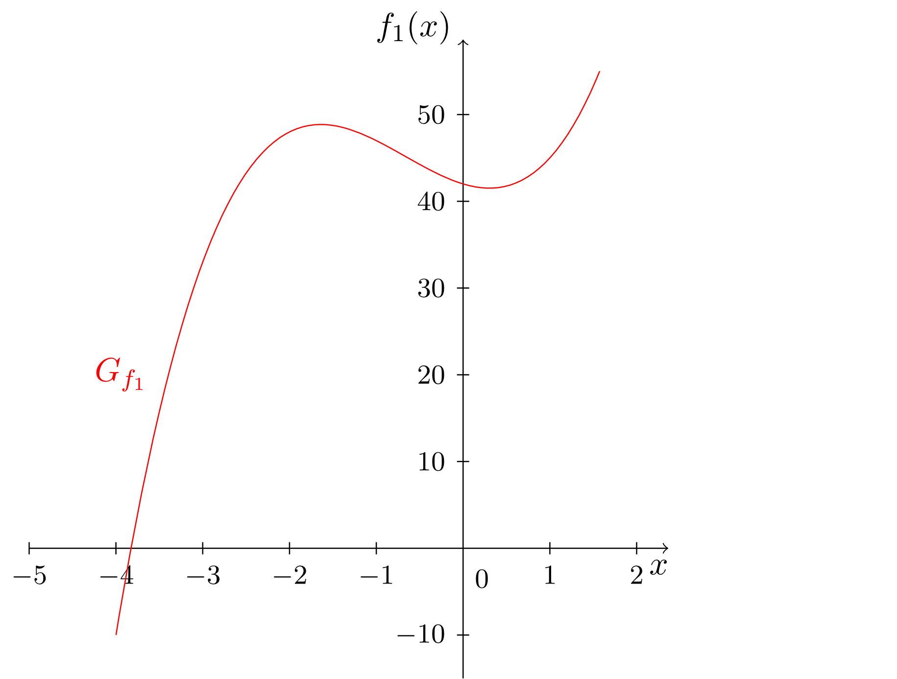
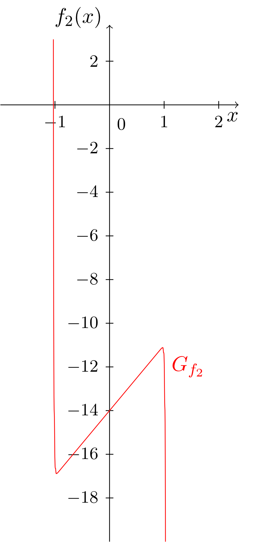
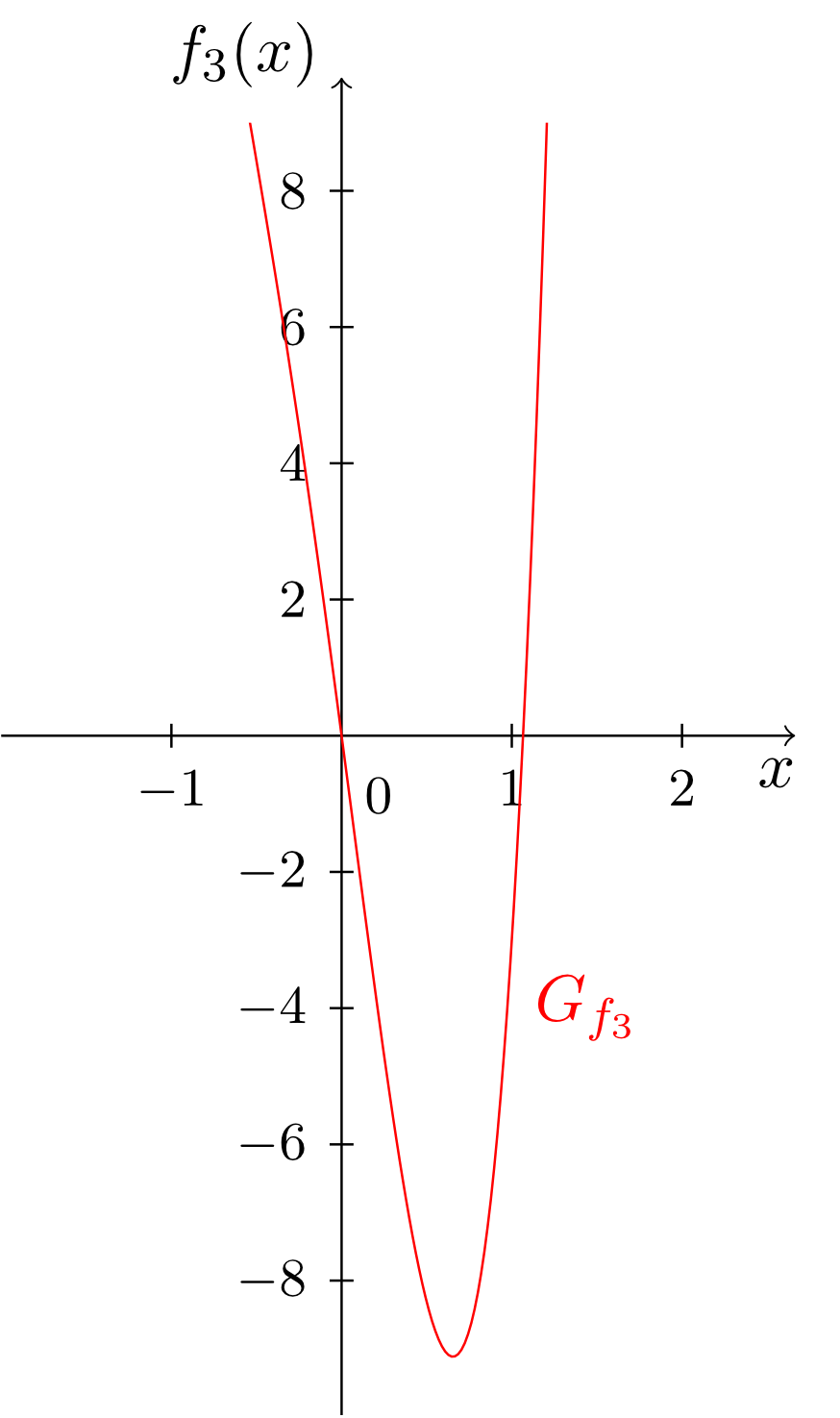
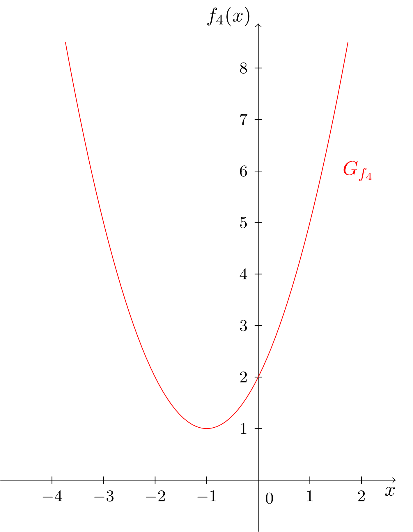
The monomials considered until now always involved only exactly one power of the independent variable. From these monomials we can easily construct more complex functions involving several different powers of the independent variable. These are sums of multiples of monomials. They are called polynomials. A few examples and their graphs are given below.
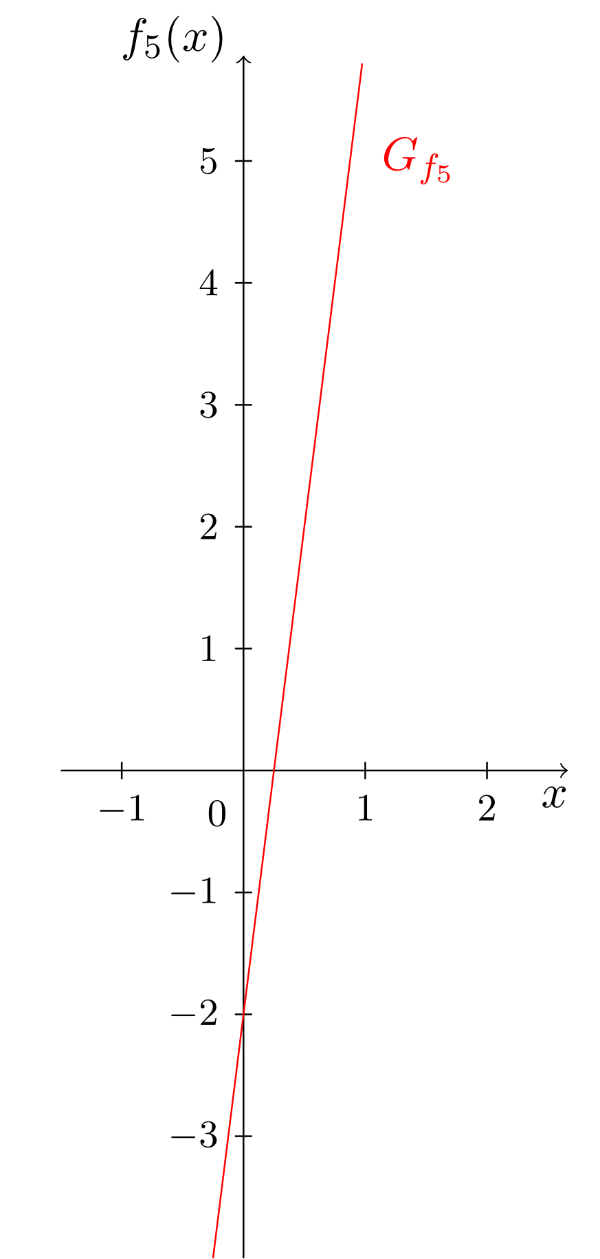
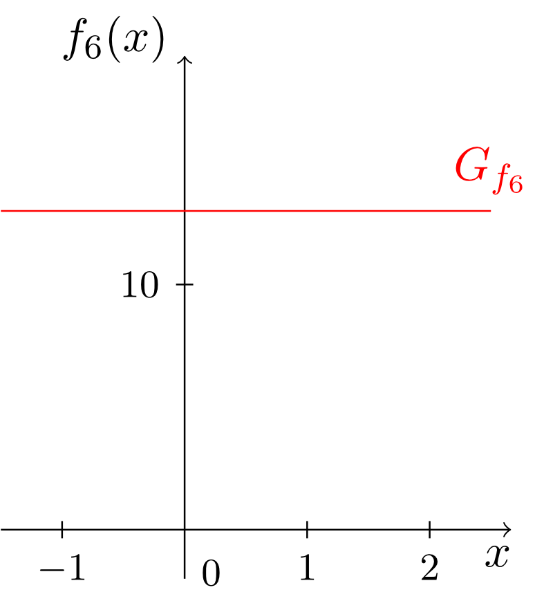
Obviously, the degree of a polynomial is determined by the monomial with highest degree. Moreover, we see that all types of functions (constant functions, linear functions and linear affine functions) studied so far - as well as the monomials - occur naturally as special cases of polynomials. Thus, the polynomials include all types of functions considered so far.
An unspecific polynomial of degree is written as follows:
Here, with are real prefactors of the individual monomials, which are called coefficients of the polynomial.
Exercise 6.2.12
What is the polynomial with the coefficients , , and , and what is its range?
The polynomial is
,
its range is .
Enter the number as pi and the range as an interval.
The polynomial is
,
its range is .
Enter the number as pi and the range as an interval.
For general polynomials, the roots are of particular interest. The roots of a polynomial can be found by solving equations of th degree. In the case of degree polynomials of degree (which are also called general parabolas), this is possible by solving a quadratic equation. In Module 2 the relevant terms and methods, i.e. completing the square, the formula, and the vertex form of quadratic expressions are explained in detail.
Example 6.2.13
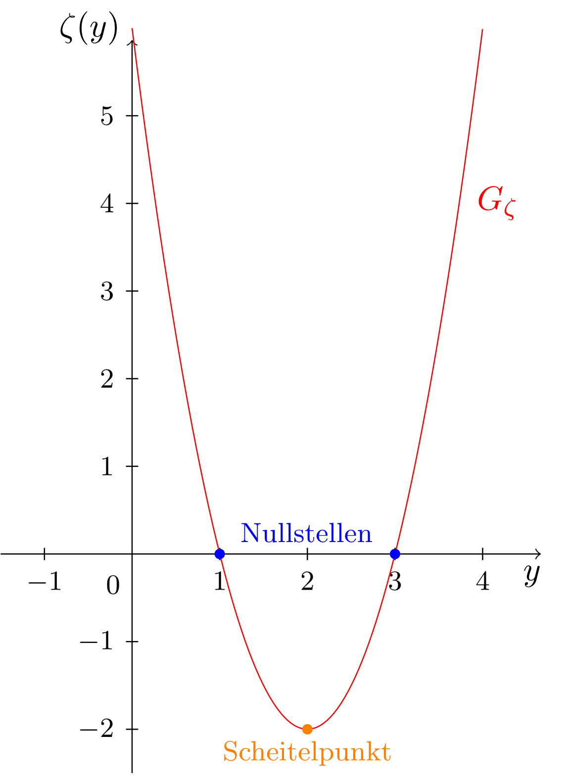
Consider the parabola
We find the roots and the vertex and then sketch the graph.
We complete the square in the mapping rule :
Thus, the mapping rule can be written as
We see that the parabola is shifted with respect to the standard parabola by units to the right and units downwards. It can be seen that the vertex is at . The roots can be calculated according to:
Finally, the graph of the function is as shown in the figure below.
