Chapter 6 Elementary Functions

Section 6.1 Basics of Functions

6.1.4 Invertability

The visualisation of a function, as for example

${\displaystyle f:\mathrm{\hspace{0.5em}\hspace{0.5em}}\{\begin{array}{ccc}\hfill ℝ& \hfill \to \hfill & ℝ\hfill \\ \hfill x& \hfill ⟼\hfill & x^2\hspace{0.5em},\hfill \end{array}}$
in form of a so-called Venn diagram (see Section 6.1.2)

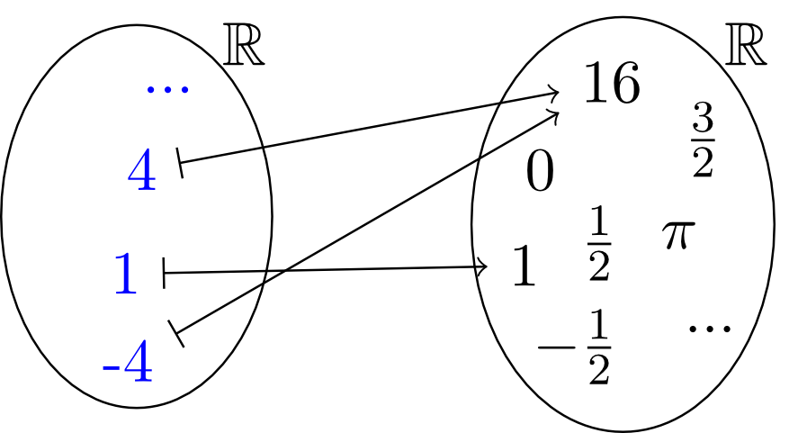
is in fact useful to understand what a function really is, but it says nothing about the special properties of the function. For this purpose, another kind of graphical representation exists, namely the representation as the graph of the function. For this representation, we draw a two-dimensional coordinate system (see Module 9) in which the numbers of the domain of the function are indicated on the horizontal axis and the numbers from the range are indicated on the vertical axis. In such a coordinate system we mark all points $(x|f(x))$ arising by the assignment of the function $x⟼f(x)$. In this case, these are all points $(x|x^2)$, i.e. $(1|1)$, $(-1|1)$, $(-\frac{\pi }{2}|\frac{{\pi }^2}{4})$, etc. This results in a curve that is called graph of $f$ and that is denoted by the symbol $G_f$:

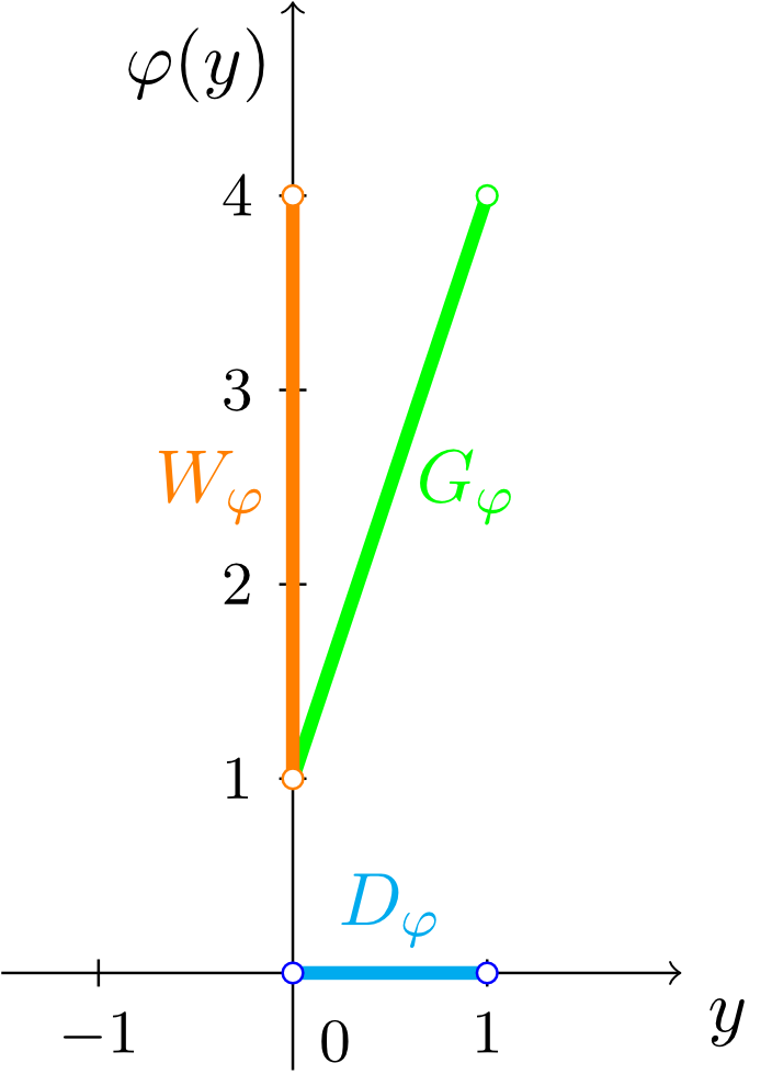
If we consider the function

${\displaystyle f:\mathrm{\hspace{0.5em}\hspace{0.5em}}\{\begin{array}{ccc}\hfill \mathbb{N}& \hfill \to \hfill & \mathbb{Q}\hfill \\ \hfill n& \hfill ⟼\hfill & \frac{n}{2}\hfill \end{array}}$
from Section 6.1.2 and its graph

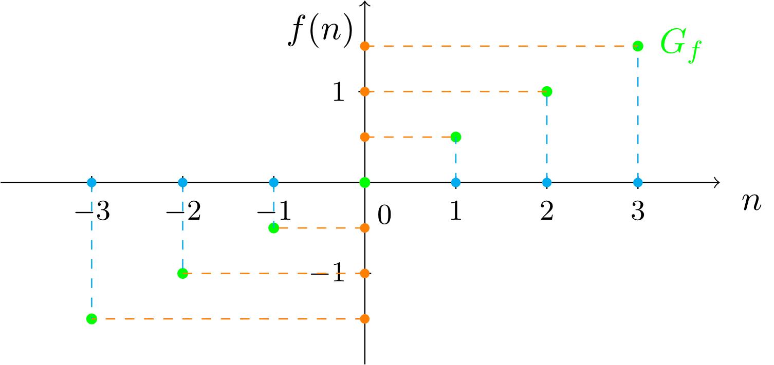
then we see that graphs not always have to be continuous curves, but also can consist, as in this case, only of single points.
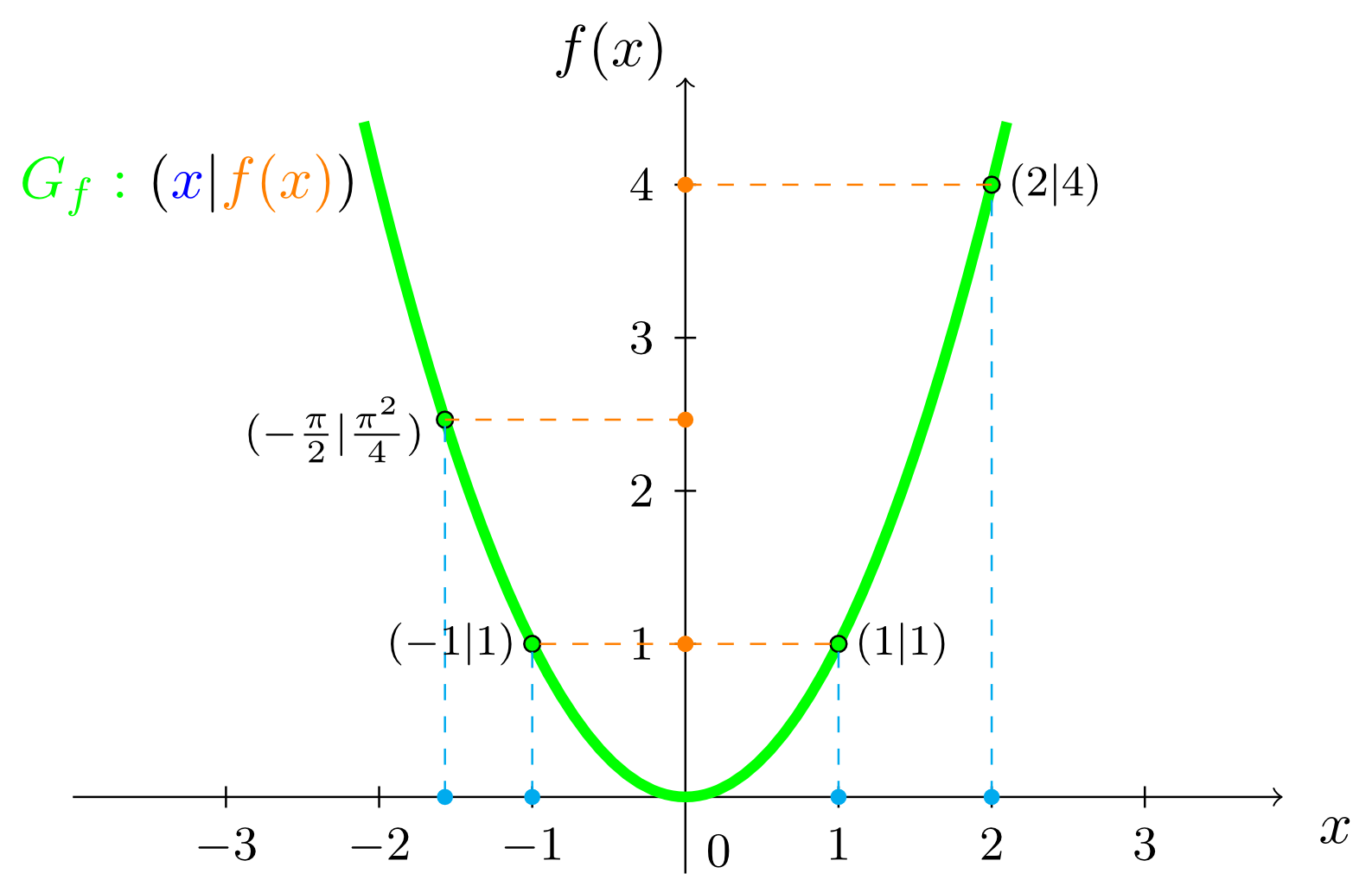
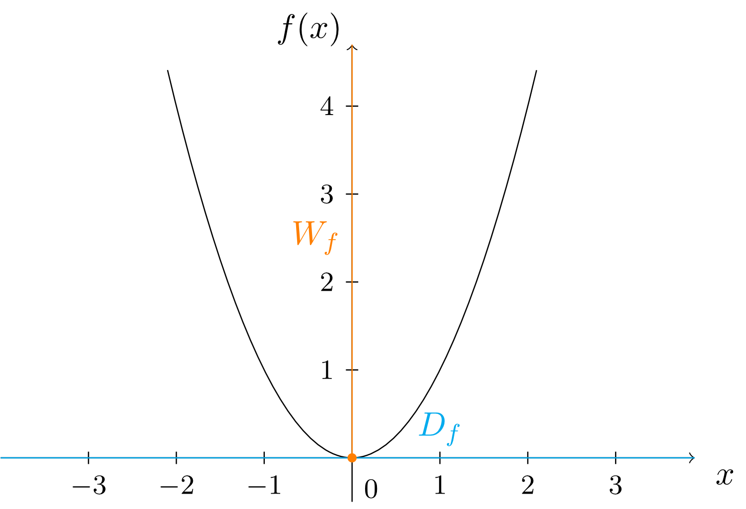
Now, from the graph we can see many basic properties of the function. Recall the function

${\displaystyle \phi :\mathrm{\hspace{0.5em}\hspace{0.5em}}\{\begin{array}{ccc}\hfill (0;1)& \hfill \to \hfill & ℝ\hfill \\ \hfill y& \hfill ⟼\hfill & 3y+1\hfill \end{array}}$
with domain $D_{\phi }=(0;1)$ and range $W_{\phi }=(1;4)$ from Section 6.1.2. If we draw its graph, then we see that the domain and the range appear on the horizontal and on the vertical axes, respectively:


Furthermore, the property of uniqueness of functions can be seen from the graph. To convince ourselves of this, we realise that a curve as shown in the figure below

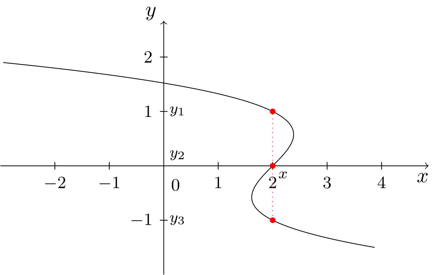
cannot be a graph of a function. For a single $x$-value in the domain, several values $y_1,y_2,y_3$ had to exist in the range. Graphs of functions indicate the uniqueness by the fact that they "cannot reverse in the horizontal direction".
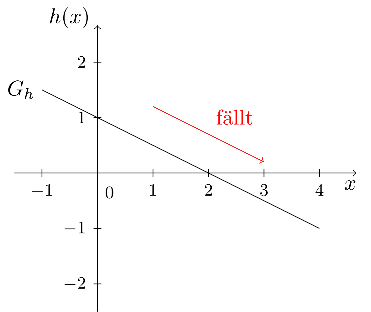
Another important property of a graph is its growing behaviour. Let us consider the function

${\displaystyle f:\mathrm{\hspace{0.5em}\hspace{0.5em}}\{\begin{array}{ccc}\hfill ℝ& \hfill \to \hfill & ℝ\hfill \\ \hfill x& \hfill ⟼\hfill & x^2\hfill \end{array}}$
and its graph.

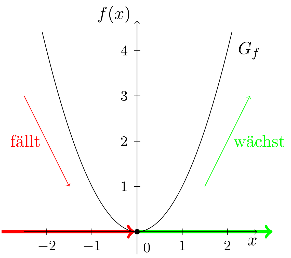
On the horizontal axis in this graph we see two regions in which the growing behaviour of the graph is different. In the region of $x$-values with $x\in (-\infty ;0)$ the graph falls, i.e. if the $x$ values increase, then the corresponding function values on the vertical axis decrease. In the region of $x$-values with $x\in (0;\infty )$ we observe the contrary behaviour. For increasing $x$-values the corresponding function values also increase: the graph rises. At the $x$-value $0\in ℝ$ the region of decreasing growing behaviour merges into the region of increasing growing behaviour. Such values will be of particular importance for the study of vertices in Section 6.2.7 and for the determination of extreme values in Module 7.
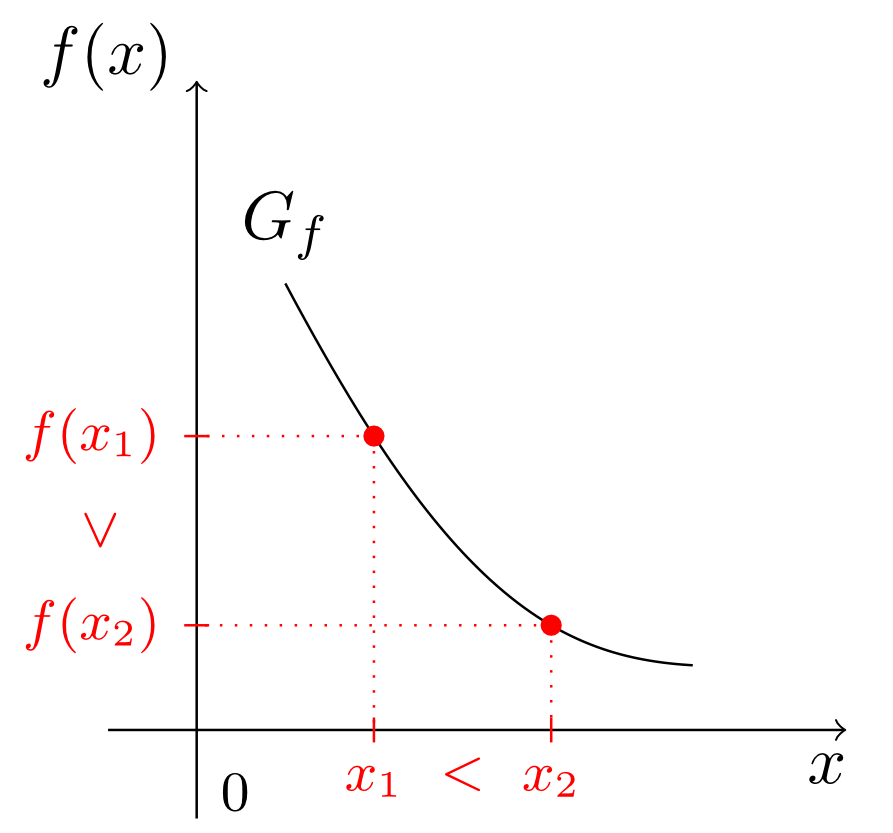
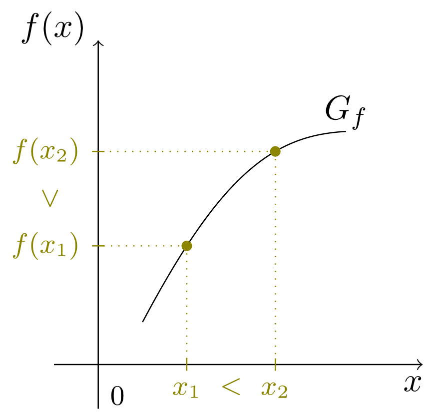
These two properties are referred to as strictly decreasing and strictly increasing, respectively, and they are defined mathematically as follows:

This is true for all functions that will be investigated throughout this module. Often, the described monotonicity properties are only true for certain regions in the functions's domain, as we have seen for the case of the standard parabola. However functions also exist which only have one of the monotonicity properties for the entire domain (see Example 6.1.16 below). In this case the entire function is called strictly increasing or strictly decreasing. A function that is either strictly decreasing or strictly increasing is simply called strictly monotonic.
A further example shows how strict monotonicity can be checked explicitly for a function by solving inequalities from Module 3.